Chapter 8

Dynamic Simulation

Every chapter until now solved for a single steady state — the plant sitting still. But plants start up, shut down, get disturbed, and are held in place by controllers. Dynamic simulation adds the one thing steady state leaves out: time.

8.1 From steady state to time

A steady-state balance says what goes in equals what goes out. A dynamic balance keeps the term steady state throws away — accumulation. For the holdup of component

i

in a unit:

\frac{dM_i}{dt} = \sum_{\text{in}} \dot n_i - \sum_{\text{out}} \dot n_i + \nu_i\, r

$M_i$: Holdup of component i in the unit (mol) — the new state variable dynamic simulation adds on top of steady state.
$\dot n_i$: Molar flow rate of component i (mol/s) in a given inlet or outlet stream.
$\nu_i$: Stoichiometric coefficient of i in the reaction (positive for a product, negative for a reactant, zero if i doesn't react).
$r$: Reaction rate (mol/s) — zero for a purely physical (non-reacting) holdup, e.g. a tank or column sump.

Now the model is a set of differential equations (one per holdup) coupled to the same algebraic equations as before (equilibrium, summation, energy) — a DAE system, integrated forward in time by an implicit solver. Set every

dM_i/dt = 0

and you're back to Chapter 1's steady state; that's not a coincidence, it's the same model with the clock stopped.

Worked example — a well-mixed tank's first-order response

Take a single holdup with no reaction:

V\,dC/dt = F\,(C_\text{in} - C)

, a first-order lag with time constant

\tau = V/F

. Say

\tau = 10

minutes and the inlet concentration steps to a new value. By hand:

\text{at } t=\tau:\quad 1 - e^{-1} = 1 - 0.3679 = 0.6321 \;\;(63.2\%\text{ of the change})

\text{at } t=4\tau:\quad 1 - e^{-4} = 1 - 0.0183 = 0.9817 \;\;(98.2\%\text{ of the change})

Hence the standard rule of thumb: a first-order holdup covers ~63% of a step change in one time constant and is effectively settled in about four — the same check applies to any tank level, column sump composition, or HX metal temperature the dynamic solver tracks.

8.2 Initialized from steady state

A dynamic run needs a consistent starting point, and the natural one is the converged steady-state solution you already have. MaximaLabs runs the dynamics from the steady-state design — no re-authoring the flowsheet — so time zero is the answer from the earlier chapters, and you watch the plant move away from it and settle back.

8.3 Control loops

The reason most plants are dynamic-but-stable is control. A feedback controller measures a process variable (PV), compares it to a setpoint (SP), and moves a manipulated variable to close the error

e = \text{SP} - \text{PV}

. The workhorse is the PID law:

u(t) = K_c\left[\,e(t) + \frac{1}{\tau_I}\int_0^{t} e(t')\,dt' + \tau_D\,\frac{de}{dt}\,\right]

$u(t)$: Controller output — the manipulated-variable signal sent to the final control element (e.g. a valve position or a heater duty).
$K_c$: Controller gain — how strongly the output reacts to a given error (proportional action).
$e(t)$: Error at time t, e = SP − PV (setpoint minus the measured process variable).
$\tau_I$: Integral time — smaller values make integral action stronger, accumulating past error faster.
$\tau_D$: Derivative time — larger values react more strongly to how fast the error is currently changing.

Worked example — why proportional-only control leaves an offset

A tank temperature loop: setpoint 350 K, measured (PV) 345 K, so

e = \text{SP} - \text{PV} = 350 - 345 = 5\ \text{K}

. With a P-only controller (

\tau_I \to \infty

, no derivative) and

K_c = 2

, the proportional term alone contributes

K_c\,e = 2 \times 5 = 10

to the output.

To keep feeding that +10 into the final control element — which is exactly what's needed to counteract a steady load — the controller must keep seeing a nonzero error. If the error ever reached zero, the output would drop back to just its bias and the load would pull the temperature away from setpoint again. So the loop settles with a permanent 5 K offset; only adding the integral term removes it (§8.6, exercise 2).

Below, a level controller on a tank is disturbed by a feed-flow step and pulls the level (PV) back to its setpoint (SP) — the classic closed-loop response. Tune the gains and you trade off speed against overshoot, exactly as on a real DCS:

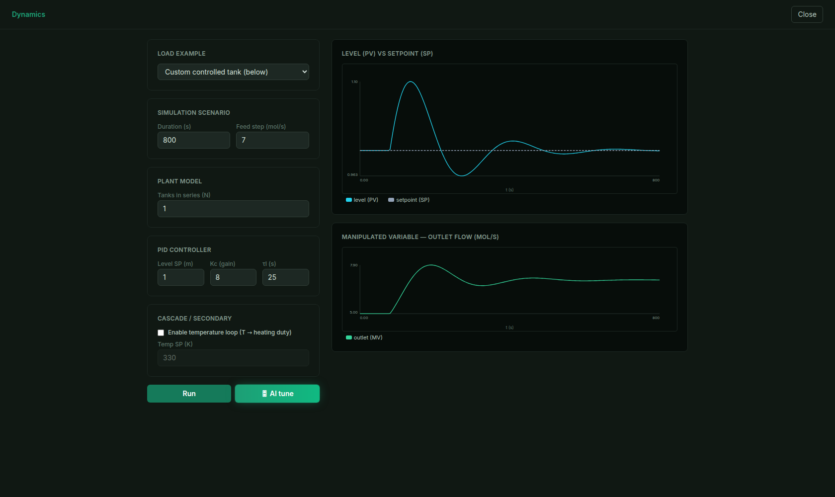
A MaximaLabs dynamic control-loop chart: tank level (PV) tracking its setpoint (SP) over time after a feed-flow disturbance, under PID control.

A PID level loop rejecting a feed-flow disturbance: the level (PV) departs from setpoint (SP) when the feed steps, then the controller drives it back. Tuning the gains trades speed for overshoot.

8.4 Running a whole flowsheet in time

Dynamics isn't only for single tanks. Switch the status-bar solve mode to Dynamic and MaximaLabs compiles any steady-state flowsheet — columns, reactors, recycle loops and all — into a DAE and integrates it from its steady-state design (no re-authoring). Pick a holdup and it charts that unit's composition or temperature vs. time; add a feed step (a flow, temperature, or composition change at a chosen instant) and you watch the disturbance propagate through the plant and settle to a new steady state.

This is the payoff of the unified model: the steady-state flowsheet, the property methods, the reactors and columns you built in the earlier chapters are exactly what runs dynamically — you add time, not a second model.

8.5 Try it

Reproduce it in your browser

1Open any converged example (e.g. the ethanol-water column) and Run it to steady state first.
2Open Simulation ▸ Dynamic simulation… for the controlled-tank scenario, set a level setpoint and a feed-flow disturbance, and Run to watch the PID loop pull the level back.
3Retune the controller gains ( $K_c$ , $\tau_I$ ) and re-run — see the response get faster but start to overshoot.
4Switch the status-bar solve mode to Dynamic to run the whole flowsheet in time and chart each holdup's transient toward steady state.

And that's the arc: build a flowsheet as a graph, pick the thermodynamics, flash it, react it, separate it, integrate its heat, analyze and optimize it — then add time. Every step used the same model, and every number came from a deterministic solver you could see the math behind. That's the whole of process simulation, and you did it in a browser.

8.6 Exercises

Practice

Work each problem yourself first, then reveal the solution to check it. Where a problem says so, reproduce it live in MaximaLabs — the solver is the answer key.

1
warm-up
A well-mixed tank of constant liquid volume $V$ has an inlet flow $F$ at concentration $C_\text{in}$ and an equal outlet flow $F$ at concentration $C$ . Write the dynamic component balance and give the time constant.
2
core
A proportional-only controller leaves a steady-state offset from setpoint. Why? And how does adding integral action remove it?
3
challenge
A step increase in feed flow disturbs a temperature loop under PID control. Describe the transient the controlled temperature follows, and how the tuning sets its shape. Reproduce a disturbance in a live loop with the Dynamics / live-PID panel.

Open the app →← Chapter 7 Chapter 9 →The Handbook