Process Analysis & Optimization
A converged flowsheet answers one question: what happens at these conditions? Real engineering asks better ones — how sensitive is the answer, what input hits a target, which design is cheapest. This chapter turns the model from a calculator into a decision tool.
7.1 Sensitivity analysis
The first question is always "what if?" A sensitivity sweep varies one input
- The k-th value of the swept input (e.g. reflux ratio) — chosen at N evenly spaced points across the range.
- The lower and upper bound of the sweep range you set.
- Number of sweep points — each one a full, independent re-solve of the flowsheet.
- The tracked output (e.g. reboiler duty) at that point — the solver's real answer, not an interpolation.
For the ethanol-water column, sweeping the reflux ratio against the reboiler duty shows the central trade-off of distillation: more reflux sharpens the separation but costs energy, and the curve tells you where the knee is. MaximaLabs runs each point as a real re-solve (an enqueued job) and plots the response:
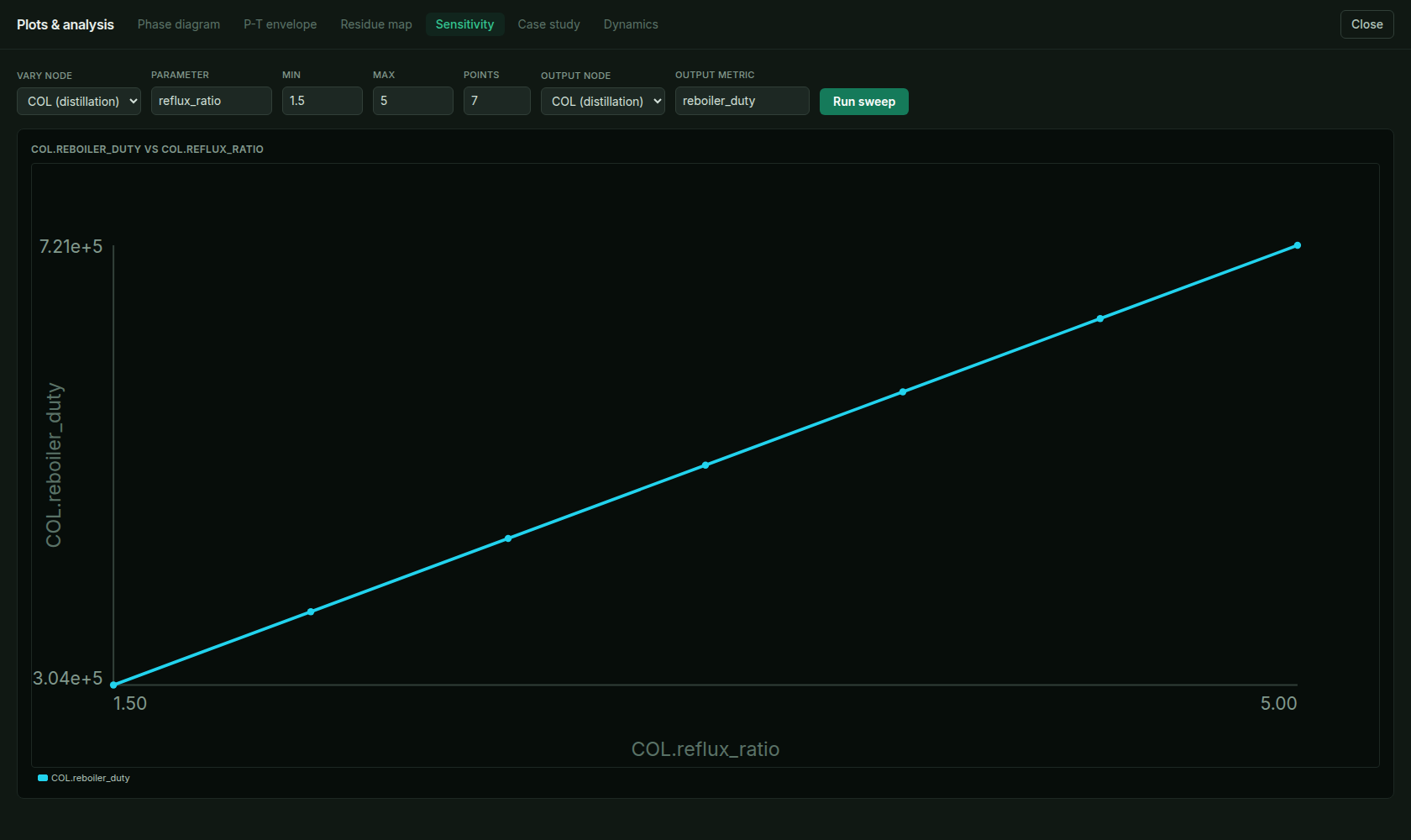
A sensitivity sweep of reflux ratio vs. reboiler duty for the ethanol-water column — every point is a full flowsheet re-solve. This is the reflux/energy trade-off, drawn.
7.2 Design specs: state the result, solve for the input
Sensitivity answers "what does this input do?" A design spec answers the inverse — "what input gives me this result?" You name a manipulated variable and a target, and the solver root-finds the input that makes the target hit its setpoint:
- The manipulated variable — a single flowsheet parameter you designate (e.g. reflux ratio).
- The target quantity as a function of that input (e.g. distillate ethanol mole fraction) — computed by a full flowsheet re-solve at each trial x.
- The setpoint you want the target to hit (e.g. 0.8).
Instead of guessing reflux ratios until the purity comes out right, you state the purity and MaximaLabs finds the reflux — the same "Design Spec" idea as Aspen, or a SimCentral adjust. Each spec reads as a sentence and reports whether it was met on the next Run:
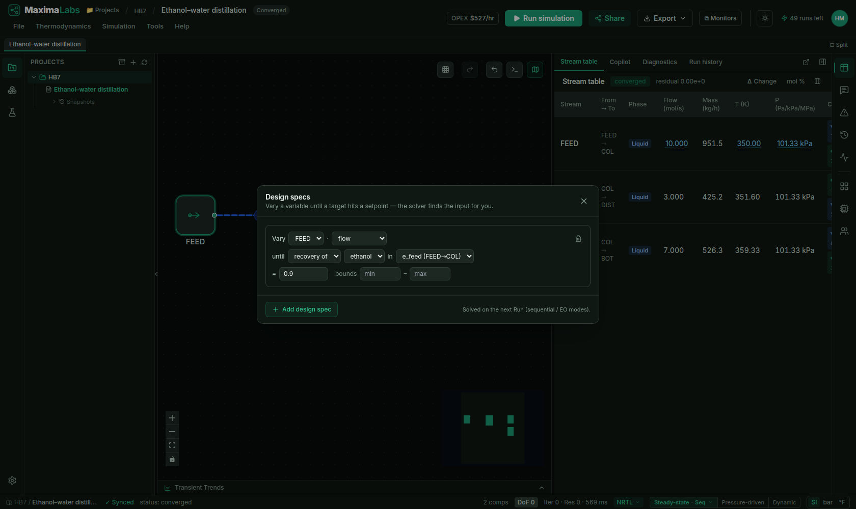
The Design Spec panel: 'vary [node · param] until [recovery/purity of …] = [setpoint]'. The solver finds the input for you and reports met / not-met with the solved value on the next Run.
7.3 Case studies
A sensitivity sweep moves one variable continuously; a case study instead evaluates a small table of named, discrete scenarios — winter vs. summer feed, three catalyst activities, a set of turndown rates — each one a full set of
- The full set of {node, param, value} overrides that define named case c (e.g. Winter feed's colder, wetter composition).
- Number of named cases (here 3: Design, Winter feed, Turndown) — discrete scenarios you actually need answers for, not a swept continuum.
- The flowsheet re-solve, read at tracked output o (e.g. distillate purity, reboiler duty).
- Number of tracked outputs (here 2: distillate purity and reboiler duty).
- The solved value of output o under case c — one cell of the results grid below.
Take the ethanol-water column and ask "what does the winter feed do to us?" — define Design (the current feed/reflux), Winter feed (colder, wetter feed composition), and Turndown (70% of design feed rate) as three cases, track distillate purity and reboiler duty as outputs, and MaximaLabs re-solves all three and returns one grid — no sweep range to define, because these are three specific, named operating points you actually need answers for, not a continuum:
| Case | Distillate purity | Reboiler duty |
|---|---|---|
| Design | 0.80 mol frac. | 1,020 kW |
| Winter feed | 0.77 mol frac. | 1,140 kW |
| Turndown (70%) | 0.83 mol frac. | 720 kW |
The pattern each row shares: colder/wetter feed costs both purity and energy (more water to reboil off), while turndown trades duty for purity in the other direction — reading that off a grid, not three separate manual runs, is the entire point of a case study. It lives on the same Plots panel as the sweep (§7.1), and reuses the identical re-solve mechanics — a case study is a sensitivity sweep over discrete named points instead of a continuous range. For four full worked case studies — reaction, separation, and economics chained across whole flowsheets, not just one column's named scenarios — see Chapter 11.
7.4 Optimization
Sensitivity and case studies explore; optimization decides. Before you can even pose the problem, you need to know whether there's a decision to make at all — the same degrees-of-freedom count from Chapter 1, applied to the whole optimization problem rather than one flowsheet solve:
- Degrees of freedom of the optimization problem — the count of variables genuinely free to be decided.
- Every unknown quantity in the problem (flows, temperatures, pressures, compositions, equipment parameters) not already fixed by a spec.
- Every material/energy balance and equilibrium relation that must hold — each one removes one degree of freedom.
Take a small piece with 3 process variables (say, a feed flow, a feed temperature, and a duty) and 2 independent equations relating them (a material balance and an energy balance):
One genuine degree of freedom remains — one decision to make (e.g. the duty), and the other two variables follow from the balances once it's chosen. This is deliberately just arithmetic to show the mechanics of the count, not a solved MaximaLabs case; the same bookkeeping applied to a real column (see Chapter 1's feed→heater→reactor degrees-of-freedom walkthrough) is what tells you whether "optimize this" even makes sense before you pose an objective.
Three cases fall out of the sign of
- The decision variables — the genuinely free variables N_f identified above (e.g. reflux ratio, feed preheat).
- The objective function being minimized (installed cost, energy, carbon — whichever you choose).
- Equality constraints — the flowsheet's own material and energy balances, which must always hold exactly.
- Inequality constraints — product specs and equipment limits the solution must not violate (e.g. purity ≥ 95%).
- Lower and upper bounds on each decision variable — the physically/operationally sane range the search stays inside.
The objective
7.5 Try it
- 1Open the ethanol-water distillation example and Run it.
- 2Open Plots ▸ Sensitivity (right rail ▸ Analysis & reports), vary the column's reflux_ratio against the reboiler_duty, and Run sweep to draw the energy trade-off.
- 3Open Simulation ▸ Design specs…, add a spec that varies reflux until the distillate ethanol purity hits a setpoint, and Run — read the solved reflux back from the met/not-met badge.
- 4Open Plots ▸ Case study, define two or three named scenarios (e.g. a colder feed temperature, a lower feed rate), track distillate purity and reboiler duty as outputs, and Run to see all cases solved side by side in one grid.
- 5Open Simulation ▸ Optimizer ▸ Optimize for lowest installed cost and watch the solver pick the decision variables — then compare its choice to the knee you saw in the sweep.
Sweep to understand, spec to hit a target, optimize to decide — all on the same converged model from the earlier chapters. Last stop: adding time, with dynamic simulation.
7.6 Exercises
Work each problem yourself first, then reveal the solution to check it. Where a problem says so, reproduce it live in MaximaLabs — the solver is the answer key.
- 1warm-upYou want the ethanol-water column's distillate to hit exactly 95 mol% ethanol. Set this up as a design spec: what is the manipulated variable, and what does the solver actually do?
- 2coreYou sweep the reflux ratio from 1.5 to 5 and plot both distillate purity and reboiler duty. What shape does each curve take, and what is the engineering takeaway?
- 3challengeNow minimize reboiler duty subject to distillate ≥ 95 mol%. Why is the purity constraint active (binding) at the optimum, and what does the optimizer move? Reproduce it in the Optimization studio on the ethanol-water column.