Chapter 5

Separation Processes

One flash (Chapter 3) buys you one stage of separation — often not enough. Stack many equilibrium stages, add reflux at the top and a reboiler at the bottom, and you get distillation: the workhorse that does most of the separation in the chemical industry. This chapter is how a column is modelled, how to read what it's doing, and how to size one fast.

5.1 A column is a stack of equilibrium stages

Picture the flash of Chapter 3 repeated on every tray: liquid falls down the column, vapor rises up it, and on each stage the two come to equilibrium — vapor enriching in the light component as it climbs, liquid enriching in the heavy component as it descends. A condenser at the top returns part of the overhead as reflux (ratio

R = L/D

), and a reboiler at the bottom boils part of the bottoms back up. The example below is the ethanol-water column from Chapter 1, now the object of study.

The MaximaLabs canvas: a FEED into a distillation column (COL) that produces a distillate (DIST) and bottoms (BOT).

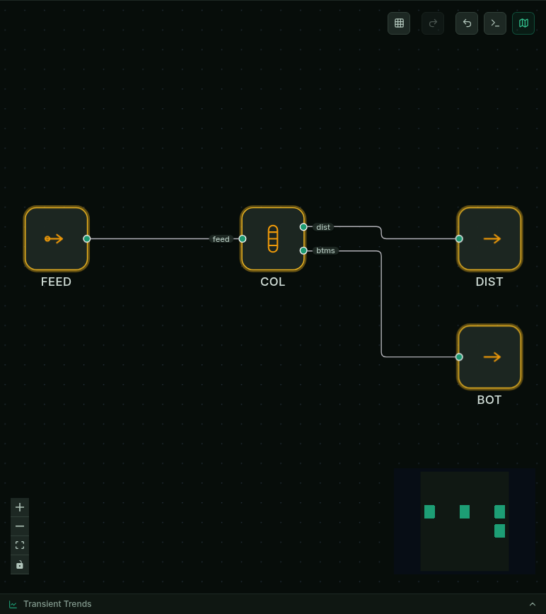
The ethanol-water distillation column: FEED → COL → distillate (DIST) + bottoms (BOT). Inside that one node is a whole stack of equilibrium stages.

5.2 The MESH equations

Rigorously, every stage

j

is described by four kinds of equation — the MESH equations — written for each component

i

\textbf{M}\;\; l_{i,j-1} + v_{i,j+1} + f_{i,j} - l_{i,j} - v_{i,j} = 0 \quad(\text{material balance})

\textbf{E}\;\; y_{i,j} = K_{i,j}\, x_{i,j} \quad(\text{equilibrium})

\textbf{S}\;\; \sum_i y_{i,j} - 1 = 0 \quad(\text{summation})

\textbf{H}\;\; L_{j-1}h^L_{j-1} + V_{j+1}h^V_{j+1} + F_j h^F - L_j h^L_j - V_j h^V_j - Q_j = 0 \;\;(\text{enthalpy})

$l_{i,j},\; v_{i,j}$: Liquid- and vapor-phase molar flow of component i leaving stage j (the unknowns the M equations balance).
$f_{i,j}$: Feed flow of component i entering stage j (zero on every stage except the feed tray).
$y_{i,j},\; x_{i,j}$: Vapor and liquid mole fraction of component i on stage j.
$K_{i,j}$: Equilibrium ratio of component i on stage j (the same K from Chapter 3's flash, evaluated at that stage's T, P, composition).
$L_j,\; V_j$: Total liquid and vapor molar flow leaving stage j.
$h^L_j,\; h^V_j$: Liquid- and vapor-phase molar enthalpy on stage j.
$Q_j$: Heat added to (or removed from) stage j — nonzero only at the condenser and reboiler for an ordinary column.

That's

M\!\times\!N

coupled nonlinear equations for an

N

-stage,

M

-component column, solved simultaneously by a Newton method — the equation-oriented idea from Chapter 1, applied inside a single unit. MaximaLabs shows you the exact set on the column's Theory tab:

$The MaximaLabs distillation column 'Theory' tab rendering the MESH equations (material balance, equilibrium, summation, enthalpy) in KaTeX with a variable legend.$

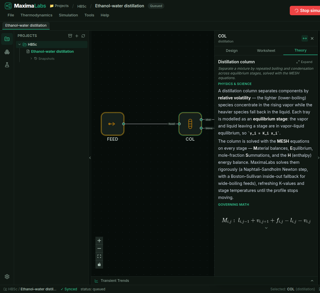
The column's 'show the math' (ParamEditor ▸ Theory): the MESH equations MaximaLabs solves on every stage, rendered in full — the same equations Aspen's RadFrac solves, here in plain view.

5.3 McCabe-Thiele: the picture behind the column

Before rigorous solvers existed, engineers sized binary columns graphically with the McCabe-Thiele construction — and it's still the clearest picture of what a column does. On the equilibrium

x\text{-}y

diagram from Chapter 2 you draw two operating lines (the mass balances above and below the feed),

y_{n+1} = \frac{R}{R+1}\,x_n + \frac{x_D}{R+1} \quad(\text{rectifying operating line})

$R$: Reflux ratio L/D — moles refluxed per mole of distillate.
$x_n,\; y_{n+1}$: Liquid composition leaving stage n and vapor composition entering it from below — successive points on the operating line.
$x_D$: Distillate composition (the line's fixed point: at x_n=x_D, y_{n+1}=x_D too).

and step off stages as a staircase between the operating lines and the equilibrium curve — each tread is one theoretical stage. MaximaLabs draws it for a solved column, actual stages and all:

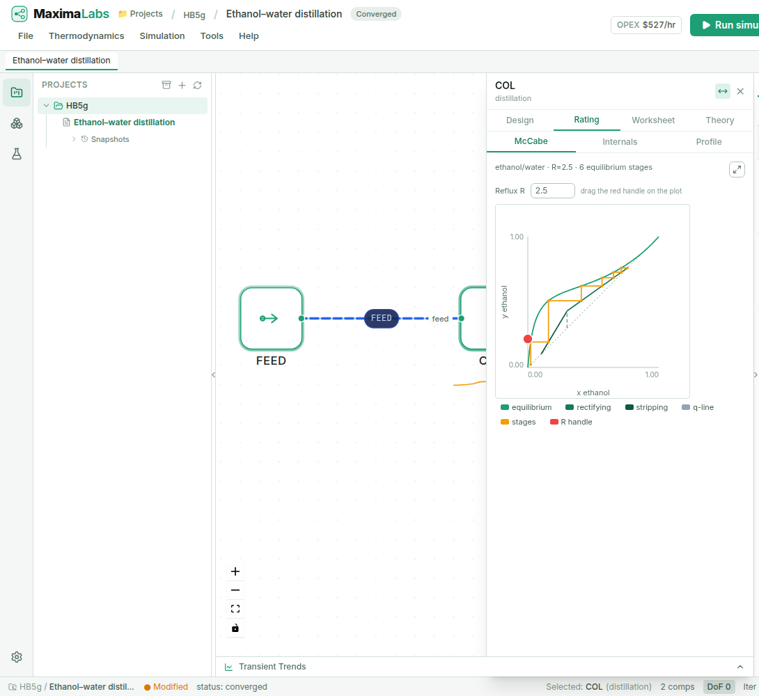
A MaximaLabs McCabe-Thiele diagram for the ethanol-water column: the equilibrium x-y curve, the rectifying and stripping operating lines, and the stepped staircase of stages between them.

McCabe-Thiele for the ethanol-water column: the equilibrium curve, the operating lines set by the reflux ratio, and the step-off staircase — one step per theoretical stage. The steps bunch up as they approach the azeotrope.

5.4 Reading the column: stage profiles

A rigorous solve gives more than top and bottom products — it gives the full internal state, stage by stage: temperature, the liquid and vapor traffic (

L_j, V_j

), and the composition on every tray. These profiles are how you diagnose a column — spot a pinch (stages doing no separation), find the real feed-stage optimum, or see a temperature break:

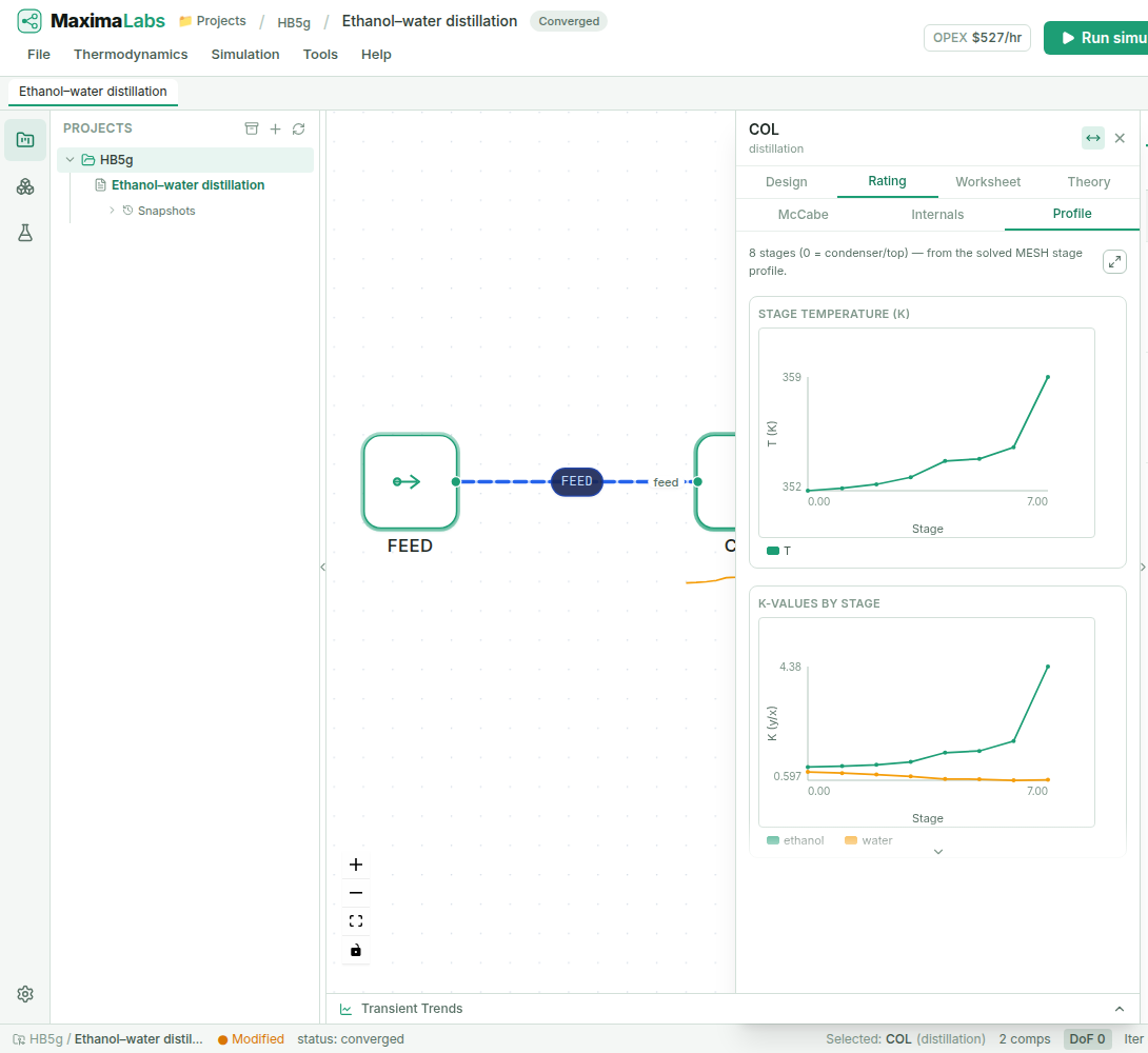
The column's stage profiles (ParamEditor ▸ Profile): temperature and internal liquid/vapor flows down the column. Where the temperature curve flattens, stages are doing little work — a pinch.

5.5 Shortcut design (Fenske-Underwood-Gilliland)

A full MESH solve needs a column to already exist. To design one — how many stages, what reflux — engineers start with the FUG shortcut (Aspen's DSTWU). Fenske gives the minimum stages at total reflux from the relative volatility

\alpha

and the desired split:

N_{\min} = \frac{\ln\!\left[\left(\dfrac{x_{LK}}{x_{HK}}\right)_{\!D}\left(\dfrac{x_{HK}}{x_{LK}}\right)_{\!B}\right]}{\ln \alpha_{LK,HK}}

$N_{\min}$: Minimum theoretical stages, at total reflux (R=infinity) — the fewest stages any design at this split could use.
$\alpha_{LK,HK}$: Relative volatility of the light key over the heavy key.
$(x_{LK}/x_{HK})_D,\;(x_{HK}/x_{LK})_B$: Light-to-heavy-key ratio in the distillate, and heavy-to-light-key ratio in the bottoms — how sharp the desired split is.

Worked example — Fenske minimum stages

\alpha = 2.4

, distillate 95 mol% light key, bottoms 5 mol% light key (the same case as §5.8's warm-up exercise):

N_{\min} = \frac{\ln[(0.95/0.05)(0.95/0.05)]}{\ln 2.4} = \frac{\ln 361}{\ln 2.4} \approx 6.7

About 7 theoretical stages at total reflux — the floor a real, finite-reflux design sits above.

Underwood gives the minimum reflux ratio — the other end of the design-space wall, where an infinite number of stages would be needed. For a multicomponent feed you first solve for the root(s)

\theta

\sum_i \frac{\alpha_i\, x_{F,i}}{\alpha_i - \theta} = 1 - q \qquad (\alpha_{HK} < \theta < \alpha_{LK})

$\alpha_i,\; x_{F,i}$: Relative volatility and feed mole fraction of component i.
$\theta$: The Underwood root(s) — a value strictly between the heavy- and light-key volatilities, solved for numerically.
$q$: Feed liquid fraction (thermal condition): q=1 saturated liquid, q=0 saturated vapor, in between a flashed feed.

where

q

is the feed's liquid fraction (thermal condition), then use

\theta

in a second summation over the distillate to get

R_{\min}

R_{\min} + 1 = \sum_i \frac{\alpha_i\, x_{D,i}}{\alpha_i - \theta}

$R_{\min}$: Minimum reflux ratio — the other design-space wall (infinite stages needed below this).
$x_{D,i}$: Distillate mole fraction of component i.

Gilliland then closes the loop: given

N_{\min}

(Fenske) and

R_{\min}

(Underwood), pick an actual operating reflux

R \approx 1.2\text{–}1.5\,R_{\min}

and read off the actual stage count

N

from an empirical correlation between the two dimensionless ratios:

\frac{N - N_{\min}}{N + 1} = 1 - \exp\!\left[\left(\frac{1+54.4X}{11+117.2X}\right)\!\left(\frac{X-1}{\sqrt X}\right)\right], \qquad X = \frac{R-R_{\min}}{R+1}

$N$: Actual stage count at the chosen operating reflux R — what the correlation solves for.
$X$: The dimensionless reflux ratio (R-R_min)/(R+1) — Gilliland's correlating variable.

Worked example — a real FUG shortcut run

A propane/n-butane depropanizer (50/50 feed, 8 atm, saturated liquid, 99% light-key recovery/99% heavy-key rejection), solved via MaximaLabs' actual shortcut solver under Peng-Robinson:

\alpha_{avg} = 2.91, \quad N_{\min} = 8.60, \quad R_{\min} = 1.01

R = 1.31\,R_{\min} = 1.31, \quad N \approx 19.1 \;\text{stages}, \quad \text{feed stage} \approx 9.6

Real solver output, not hand-picked — this is exactly what the Shortcut column tool below returns for this feed.

Fenske → Underwood → Gilliland is the classic one-shot sequence: three cheap algebraic equations instead of a full MESH solve, good enough to size a column before committing to the rigorous model. MaximaLabs exposes exactly this as the Shortcut column tool (Analysis & reports ▸ Engineering analysis) — enter the light/heavy key recoveries and it returns

N_{\min}

R_{\min}

, and the Gilliland-estimated actual

N

in one call, the same three equations above.

5.6 The wall: azeotropes

Distillation separates by relative volatility, so where volatility vanishes —

\alpha \to 1

, the azeotrope — an ordinary column stalls. On the McCabe-Thiele picture the staircase can't step past the point where the equilibrium curve meets the diagonal; ethanol-water pinches at about 89 mol% ethanol no matter how many trays you add. Breaking that wall (pressure-swing, entrainer, extractive or azeotropic distillation) is its own craft — and exactly the sort of thing you'd ask the copilot to set up.

5.7 Try it

Reproduce it in your browser

1Open the ethanol-water distillation example and Run it.
2Click the COL node and open the McCabe tab to see the staircase, then Profile for the stage-by-stage temperature and flows, and Theory for the MESH equations.
3Change the reflux ratio and re-run — watch the operating lines tilt on McCabe-Thiele and the distillate purity move. More reflux, sharper split, more reboiler duty.
4Move the feed stage and re-run — the profiles show whether you've placed it well (a smooth composition front) or badly (a kink and wasted stages).
5Try pushing the distillate purity past ~89% ethanol — it won't go, because the azeotrope caps it. That's §5.6, live.

A column is just Chapter 3's flash, stacked and wired with reflux and reboil — and everything you've learned so far (thermodynamics, flash, the equation-oriented solve) is doing the work inside that one node.

5.8 Exercises

Practice

Work each problem yourself first, then reveal the solution to check it. Where a problem says so, reproduce it live in MaximaLabs — the solver is the answer key.

1
warm-up
Estimate the minimum number of stages (total reflux) with the Fenske equation for a separation with relative volatility $\alpha = 2.4$ , a distillate at 95 mol% light key, and bottoms at 5 mol% light key.
2
core
On a McCabe-Thiele diagram, what happens to the number of stages as the reflux ratio $R$ increases, and what do you pay for it? Name the two limits $R \to \infty$ and $R \to R_\text{min}$ .
3
challenge
Push the ethanol-water column toward a 99 mol% ethanol distillate and it stops improving. Explain what the stage profile and McCabe-Thiele diagram are showing, and name three ways to actually get past it.

Open the column example →← Chapter 4 Chapter 6 →The Handbook