Chapter 1

Simulation Fundamentals

Before any thermodynamics or unit-operation detail, a process simulator has to answer one question: given a set of connected equipment and some specifications, what are all the stream flows, temperatures, pressures, and compositions? This chapter is the machinery that answers it — the same machinery under Aspen Plus and HYSYS, but in MaximaLabs it's not hidden. You can watch it work.

1.1 A flowsheet is a graph

A steady-state model is a directed graph: nodes are unit operations (feeds, reactors, columns, exchangers, products) and edges are the streams that carry material between them. Every stream is the same object everywhere in MaximaLabs — flow, temperature, pressure, composition, phase, enthalpy, entropy — so the simulator, the cost estimator, and the reports all read one representation.

The example below is a minimal loop: a feed mixes with a recycle, is heated, and split — part leaves as product, part returns. Notice the orange tear badge on the returning stream; we'll come back to why it's marked (§1.4).

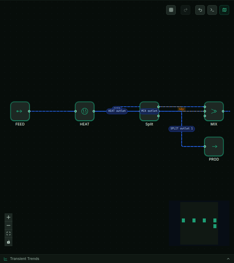
A recycle loop on the MaximaLabs canvas: FEED → MIX → HEAT → Split, with one Split outlet returning to the mixer (marked 'tear') and one leaving as product.

The reference 'Recycle loop' example on the MaximaLabs canvas. The returning stream is flagged as the tear (orange badge) — the edge the solver cuts to break the cycle.

1.2 Two ways to solve it: sequential-modular vs. equation-oriented

There are two classical strategies for solving that graph, and MaximaLabs implements both — you pick from the Steady-state strategy menu in the status bar.

Sequential-modular (SM). Each unit is a self-contained module: given its inlets and parameters, it computes its outlets. The solver visits units in topological order, passing streams forward. It's robust and easy to reason about — but a recycle creates a cycle, so there's no "first" unit; SM has to guess a stream, iterate, and converge (§1.4–1.5).

Equation-oriented (EO). Instead of marching unit by unit, EO collects every model equation for the whole flowsheet into one large system and solves it simultaneously with a Newton method:

F(x) = 0, \qquad x_{k+1} = x_k - J(x_k)^{-1} F(x_k), \quad J = \frac{\partial F}{\partial x}

$x$: The stacked vector of every unknown stream variable in the whole flowsheet (flows, temperatures, pressures, compositions) — everything the solver has to find at once.
$F(x)$: The stacked vector of every model equation (material balances, energy balances, equilibrium relations, summation constraints) evaluated at the current guess x — zero exactly when x is the converged solution.
$J$: The Jacobian — the matrix of every equation's sensitivity to every unknown (∂Fᵢ/∂xⱼ), rebuilt (or approximated) at each Newton step.
$x_k,\; x_{k+1}$: The unknown vector at iteration k and the next, improved iteration — Newton's method repeats this update until F(x) is below tolerance.

Here

x

stacks all the unknown stream variables and

F

stacks all the material balances, energy balances, equilibrium and summation relations. A recycle is no longer special — it's just a few more equations in the same system. This is the approach AVEVA SimCentral, gPROMS, and IDAES use, and it's why tightly-coupled recycles that crawl in SM converge cleanly in EO.

Worked example — the ammonia loop's EO system (§1.6)

For the high-recycle ammonia loop below, MaximaLabs' plant-wide EO mode stacks

x

and

F(x)

into a system with 28 unknowns and 28 residual equations (the same square system shown in §1.3's Solver-math screenshot) and solves it in one simultaneous Newton solve — versus the ~78 tear passes the sequential-modular strategy needs for the identical flowsheet (§1.5–1.6).

MaximaLabs Steady-state strategy menu showing Seq (sequential-modular, Wegstein recycle tearing), Tear-EO, EO (plant-wide equation-oriented), and Symbolic EO; the status bar shows a DoF 0 pill and iteration/residual readout.

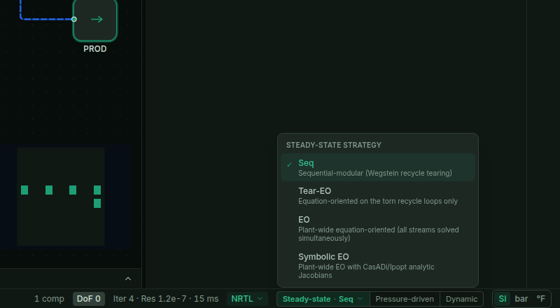
The strategy menu: Sequential-modular, Tear-EO (EO only on the torn loops), plant-wide EO, and Symbolic EO (CasADi/Ipopt analytic Jacobians). The status bar carries the live DoF pill and iteration/residual readout.

1.3 Degrees of freedom

A model is solvable only if it's square — as many independent equations as unknowns. The degrees of freedom are

N_{\text{DOF}} = N_{\text{variables}} - N_{\text{equations}}

$N_{\text{variables}}$: Total unknown stream/unit variables in the flowsheet (every flow, temperature, pressure, and composition not yet fixed by a spec).
$N_{\text{equations}}$: Total independent model equations (material balances, energy balances, equilibrium/summation relations) contributed by every unit op.
$N_{\text{DOF}}$: Degrees of freedom — the count of variables left over once the equations are subtracted. Zero means the model is exactly solvable ("square").

N_{\text{DOF}} > 0

the flowsheet is under-specified (you must fix more variables); if

N_{\text{DOF}} < 0

it's over-specified (a spec has to give). MaximaLabs computes this structurally from the graph and shows it live as the DoF pill in the status bar — so you see under/over-specification before you ever hit a cryptic solver failure. The Solver-math panel makes it concrete: the equation-oriented system for the recycle example below is exactly square (28 unknowns, 28 residual equations, DoF 0), and every residual is labelled by the unit and the balance it enforces.

Worked example — the recycle-loop's DoF count

The Solver-math ▸ Structure screenshot below reads it directly:

N_{\text{variables}} = 28

N_{\text{equations}} = 28

, so

N_{\text{DOF}} = 28 - 28 = 0

— exactly square, well-posed, no missing or redundant specs. That's the number that lets the solver even attempt a solve.

MaximaLabs Solver Diagnostics 'Structure' tab: 28 unknowns, 28 residual equations, degrees of freedom 0, well-posed 'square'; a 28×28 Jacobian sparsity grid; and a list of residual equations labelled by unit (MIX/REACTOR/CHILL) and type (component material balance, energy balance).

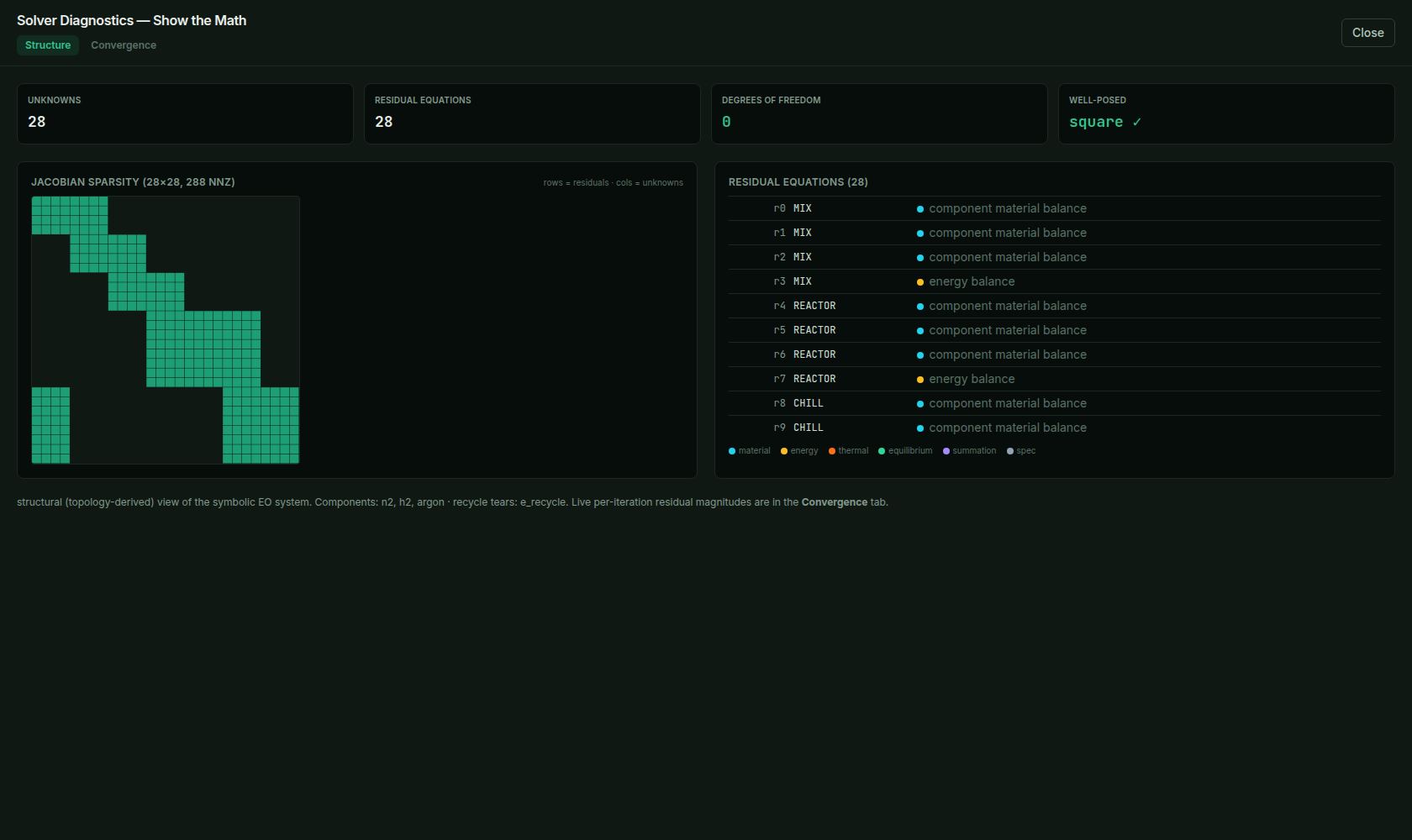
Solver-math ▸ Structure: the whole equation-oriented system laid bare — 28 unknowns = 28 equations ⇒ DoF 0 (square, well-posed), the Jacobian sparsity pattern, and each residual tagged material/energy/equilibrium/summation. Aspen solves the same system; here you can see it.

1.4 Recycles and tear streams

A recycle makes the graph cyclic, so sequential-modular can't just march forward — computing the mixer needs the recycle stream, but computing the recycle stream needs everything downstream of the mixer. The classic fix is tearing: cut one edge in the cycle (the tear stream), guess its values, march around the loop, and compare the value that comes back with the guess. The mismatch is the tear residual:

r = x_{\text{calc}} - x_{\text{guess}} \;\to\; 0

$x_{\text{guess}}$: The tear stream's assumed values (flow, T, P, composition) at the start of a pass — the guess that lets sequential-modular execution start despite the cycle.
$x_{\text{calc}}$: What that same stream computes out to after marching all the way around the loop once with that guess.
$r$: The tear residual — the gap between what was guessed and what came back. The solver keeps passing until r is below tolerance.

MaximaLabs picks the tear automatically and marks it on the canvas (the orange badge you saw in §1.1), then iterates until the residual is below tolerance. You can also pin the tear's initial guess yourself for a hard-to-start loop.

Worked example — the tear residual, ammonia loop

§1.5–1.6's high-recycle ammonia loop starts its first tear pass with residual

r \approx 7\times10^{-2}

(the initial guess is far from the real recycle composition) and Wegstein-accelerated passes drive it down to

r \approx 9.01\times10^{-7}

after ~78 passes — the point at which MaximaLabs calls the loop converged.

1.5 Convergence: direct substitution and Wegstein

Marching around a torn loop is a fixed-point iteration

x_{k+1} = g(x_k)

, where

g

is "go around the loop once." The simplest scheme, direct substitution, just feeds the result back in — but for a tightly-coupled loop it can crawl or oscillate. Wegstein acceleration fixes that by extrapolating each component from the last two passes:

s = \frac{g(x_k) - g(x_{k-1})}{x_k - x_{k-1}}, \qquad q = \frac{s}{s - 1}

x_{k+1} = q\, x_k + (1 - q)\, g(x_k)

$g(x_k)$: One trip around the torn loop starting from the current guess x_k — the same "march the loop once" operation direct substitution uses on its own.
$s$: The observed local slope of g between the last two passes — how sensitive the loop's output is to its input, estimated numerically rather than assumed.
$q$: The Wegstein extrapolation factor built from s — near 0 behaves like plain direct substitution, negative q overshoots deliberately to escape a slow crawl.
$x_{k+1}$: The next guess, blended between the raw substitution result g(x_k) and the current x_k by q — this is what replaces plain direct substitution.

The high-recycle ammonia loop below has a recycle-to-fresh ratio of about 5:1 — a genuinely stiff loop. In sequential-modular mode MaximaLabs tears it and takes ~78 Wegstein passes to drive the residual from

7\times10^{-2}

down to

9\times10^{-7}

. The Solver-math ▸ Convergence tab plots that trajectory on a log scale, so "did it converge, and how fast" is something you see, not guess:

Worked example — Wegstein on the ammonia loop

Same loop as above:

78

Wegstein-accelerated passes take the scaled tear residual from

\approx 7\times10^{-2}

to a final

9.01\times10^{-7}

. Plain direct substitution (

q=0

always) would need many more passes on a loop this stiff — extrapolating with the observed slope s is what buys the speed-up.

MaximaLabs Solver Diagnostics 'Convergence' tab: method Wegstein, 78 iterations, final residual 9.01e-7, outcome converged; a log-scale plot of scaled residual vs iteration falling from ~7e-2 to ~9e-7 over 78 steps.

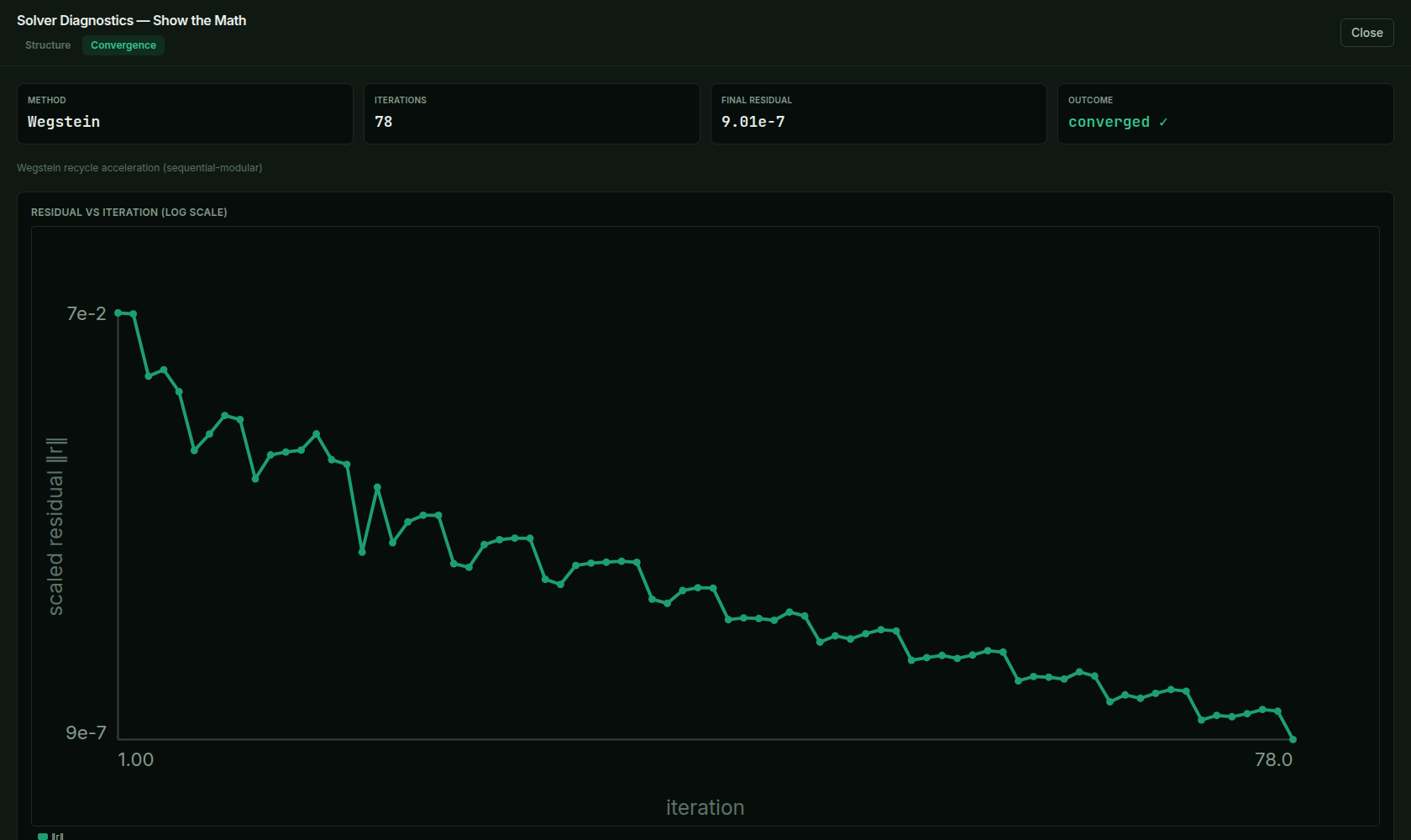
Solver-math ▸ Convergence for the ammonia loop in sequential-modular mode: 78 Wegstein iterations, residual driven to 9.01×10⁻⁷. The same loop in EO mode closes all ~35 streams in one Newton solve — same answer, different path.

1.6 Worked example: solve one loop two ways

Put it together on the high-recycle ammonia synthesis loop — fresh syngas (N₂ + 3H₂, with argon inert) mixes with a large recycle, reacts ~10% per pass, chills so ammonia condenses out as product, and the unreacted gas recycles, with a small purge to bleed the argon. It's the canonical case where solution strategy actually matters.

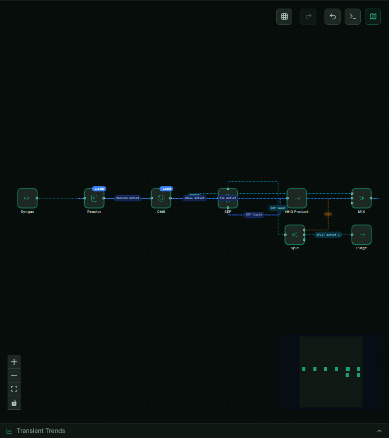
MaximaLabs canvas: the high-recycle ammonia synthesis loop — Syngas feed → Reactor (−2.2 MW) → Chill (−2.1 MW) → separator/recycle.

The high-recycle ammonia loop example, converged, on the canvas.

Reproduce it in your browser

1Open the example directly: high-recycle ammonia loop (or use the app's example gallery).
2Leave the strategy on Steady-state · Seq (the status-bar toggle) and click Run simulation. Watch the iteration/residual readout tick — this loop takes tens of tear passes.
3Open Solver math (right rail ▸ Analysis & reports) and switch to the Convergence tab to see the Wegstein residual trajectory, then Structure to see the square DoF-0 system and Jacobian.
4Now change the strategy to EO (Steady-state ▾ ▸ EO) and Run again. It reaches the same converged answer in a single simultaneous Newton solve instead of ~78 tear passes — the point of the chapter is the path, not the result.
5Read the converged stream table (right panel) and confirm the mass balance closes around the loop, argon and all.

That's the whole fundamentals loop: build a graph, check it's square, tear and converge the recycles (or solve everything at once), and read the answer. Every later chapter — thermo, reactors, distillation — is a richer node inside this same machine.

1.7 Exercises

Practice

Work each problem yourself first, then reveal the solution to check it. Where a problem says so, reproduce it live in MaximaLabs — the solver is the answer key.

1
warm-up
A flowsheet runs feed → mixer → reactor → separator, and the separator sends a product out while recycling its other outlet back to the mixer. How many streams must the sequential-modular solver tear to compute the loop, and which one?
2
core
You draw feed → heater → reactor with the feed fully specified, and the degrees-of-freedom indicator reads −1 (under-specified). What single spec is missing, and what are your two choices for it?
3
challenge
A recycle carries five units of flow back for every one unit of fresh feed (recycle ratio ≈ 5). Explain why sequential-modular needs many tear passes to converge this loop while equation-oriented solves it in a single Newton solve — then watch it in the high-recycle ammonia example.

Try the recycle loop →Chapter 2 →Back to the Handbook