Thermodynamic & Physical Property Models
Chapter 1 solved the flowsheet as a graph. But every unit in that graph — every flash, column stage, and reactor outlet — is only as correct as the property model behind it. Choosing that model is the single most consequential decision in a simulation, and the one most likely to be wrong. This chapter is how you choose, and how MaximaLabs helps you get it right.
2.1 The most important choice you make
The same flowsheet, solved with two different property methods, can give two completely different answers — not slightly different, qualitatively different. The textbook case is ethanol–water: it forms an azeotrope at about 89 mol% ethanol, a hard ceiling that ordinary distillation cannot cross. A model that captures the strong non-ideality of the liquid (an activity-coefficient model) predicts that azeotrope; a bare cubic equation of state, tuned for hydrocarbons, does not — so it will happily (and wrongly) report a column reaching 99.9% ethanol overhead. Same column, same specs; the thermodynamics decide whether the answer is physical.
2.2 Equations of state
An equation of state (EoS) relates pressure, volume, and temperature for both phases from one set of parameters. The workhorses are the cubics — Peng-Robinson (PR) and Soave-Redlich-Kwong (SRK):
- Pressure, temperature, and molar volume — the three state variables the EoS relates.
- Universal gas constant.
- Peng-Robinson pure-component energy and co-volume parameters, computed once from each component's critical temperature/pressure and acentric factor.
- A temperature-dependent correction factor on a, fit so the EoS reproduces the pure component's own vapor-pressure curve near its critical point.
The EoS gives fugacity coefficients
- Fugacity coefficient of component i in the vapor and liquid mixture — both computed from the same EoS at the mixture's T, P, and composition, so no separate liquid-phase model is needed.
- Vapor- and liquid-phase mole fraction of component i.
- Equilibrium ratio K_i = y_i/x_i, fixed once the fugacities of both phases match.
Cubics are the right default for non-polar, hydrocarbon, and high-pressure gas systems — natural gas, refinery cuts, compressors. MaximaLabs ships PR and SRK plus more specialized equations of state (PC-SAFT, CPA for associating fluids, GERG-2008 for LNG). You pick the property method from the status bar; the menu spans equations of state, activity models, electrolytes, steam, and polymer models:
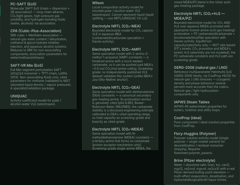
The property-method menu (status-bar thermo pill), scrolled to show the breadth beyond the cubics — SAFT-family equations of state, activity models (UNIQUAC, Wilson), electrolytes, steam tables, and a polymer model — each with what it's for. Peng-Robinson, SRK, and NRTL sit at the top of the same list; switching any of them re-solves the flowsheet.
2.3 Activity-coefficient models
For a strongly non-ideal liquid — alcohols, water, acids, anything with hydrogen bonding — the right tool is an activity-coefficient model. Here the liquid non-ideality lives in an activity coefficient
- Vapor- and liquid-phase mole fraction of component i.
- Vapor-phase fugacity coefficient of i (≈1 near atmospheric pressure, where this method is normally used).
- System (total) pressure.
- Liquid activity coefficient of i — the non-ideality correction the activity model below supplies; 1 is the ideal (Raoult's-law) limit.
- Pure-component vapor pressure of i at the mixture temperature T.
The default in MaximaLabs for polar systems is NRTL (Non-Random Two-Liquid), whose activity coefficient for component
- Activity coefficient of component i being solved for.
- Liquid mole fractions — j, k, m range over every component (the sums); i is the one component gamma is evaluated for.
- Dimensionless NRTL interaction energy for the ordered pair i,j (asymmetric — tau_ij is not tau_ji).
- NRTL local-composition weighting factor for the pair i,j — how strongly j clusters around i relative to i itself.
- Non-randomness parameter for the pair (a third fitted constant, often held near 0.2-0.3 across many families rather than regressed).
- The two fitted binary interaction constants — a is temperature-independent, b/T carries the temperature dependence.
- Temperature (K).
The binary interaction parameters
MaximaLabs' pinned ethanol(1)-water(2) NRTL parameters (regressed to published VLE data):
Both exceed 1 — a positive deviation from Raoult's law, the hydrogen-bonding non-ideality that eventually produces the ethanol-water azeotrope (§2.5). A cubic EoS with no activity model built in cannot generate this.
2.4 The rest of the activity-model family
NRTL isn't the only local-composition model, and it isn't predictive — every one of these needs fitted binary parameters. Four more are worth knowing by their actual equations, not just their names, because each makes a different trade between simplicity, physical grounding, and whether it needs data at all.
Van Laar is the oldest of the family — built directly on the van der Waals equation for regular solutions, two parameters, no temperature dependence. For a binary:
- Excess Gibbs energy of mixing (J/mol) — the departure from an ideal solution.
- Liquid mole fractions of components 1 and 2.
- Gas constant and temperature (van Laar's constants carry no further T dependence themselves).
- The two fitted, temperature-independent van Laar binary constants.
which splits into the two per-component activity coefficients MaximaLabs actually evaluates:
- Activity coefficients of components 1 and 2.
- Same two fitted constants as above — note the asymmetry: A_12 weights gamma_1 with A_21, and vice versa.
- Liquid mole fractions.
Its simplicity is also its limit — no temperature dependence means it can't track VLE over a wide range, but it's cheap to fit and still shows up for quick screening. It's a real, selectable MaximaLabs thermo package (
MaximaLabs' pinned ethanol(1)-water(2) van Laar constants:
Close to NRTL's 1.423 / 1.327 at this one composition — the two-constant fit's known weakness only shows up once you sweep across the full composition range and compare azeotrope location, not at a single point.
Wilson introduced local composition — the idea that the composition immediately around a molecule differs from the bulk because of energetic preference — which every model after it (NRTL, UNIQUAC) inherits:
- Activity coefficient of component 1 (ethanol here); gamma_2 follows the same form with subscripts 1 and 2 swapped.
- Liquid mole fractions.
- Wilson local-composition parameters, Lambda_ij = (v_j/v_i)·exp(-a_ij/T), from the pure-liquid molar volumes v_i and two fitted binary energies a_ij.
Wilson fits VLE well with only two parameters, but structurally cannot predict liquid-liquid splitting — for that you need NRTL or UNIQUAC.
MaximaLabs' pinned molar volumes
Again close to NRTL/Van Laar at this composition — all four local-composition models agree reasonably well near the middle of the range; they diverge more sharply near the azeotrope, which is exactly why MaximaLabs validates each against the same published data rather than trusting any one model's equation alone.
UNIQUAC (UNIversal QUAsi-Chemical) splits the excess Gibbs energy into a combinatorial term (molecule size/shape, from pure-component data alone) and a residual term (the energetic interactions, from two fitted parameters per pair):
- Combinatorial part of the excess Gibbs energy — accounts for molecule size/shape differences alone, from pure-component data, independent of energetics.
- Liquid mole fractions.
- Segment (volume) fractions, from r_i below.
- Surface-area fractions, from q_i below.
- Pure-component surface-area parameters.
- Lattice coordination number, fixed at 10 in MaximaLabs' implementation.
- Residual part of the excess Gibbs energy — the energetic contribution, carrying the two fitted binary parameters.
- UNIQUAC binary interaction parameters (below), asymmetric between the two directions.
- Surface-area fractions, same as above.
- Pure-component surface-area parameters.
where the segment fraction
MaximaLabs' pinned van der Waals parameters
A fourth independent confirmation, within a few percent of NRTL/Van Laar/Wilson at this composition — the four models are built on different assumptions but agree closely away from the azeotrope, which is exactly the region where the choice of model matters least.
UNIFAC (UNIversal Functional Activity Coefficient) is the predictive answer to "what if I have no binary data at all": it reuses UNIQUAC's exact combinatorial/ residual form, but builds
- Molecule i's overall volume and surface-area parameters — the same r_i, q_i UNIQUAC's equations use, now built up rather than looked up.
- Number of group k that molecule i contains (an integer count from its structure — e.g. ethanol has one -CH3, one -CH2-, one -OH).
- Tabulated volume/area parameters for functional group k, from the UNIFAC group table — not fitted per molecule or per pair.
- Residual (energetic) part of component i's activity coefficient.
- Count of group k in molecule i, same as above.
- Group k's activity coefficient evaluated in the actual mixture (all groups from every component, pooled).
- Group k's activity coefficient evaluated in a reference solution of pure component i — subtracting this out is what makes the term vanish for a molecule made of only one group type.
where
Run MaximaLabs' original-UNIFAC group decomposition on the same ethanol-water feed,
Compare that to NRTL's regressed 1.423 / 1.327 above — UNIFAC lands within about 2% having seen zero data for this specific pair, which is why it's the property estimator's fallback for an uncataloged mixture rather than a guess.
2.5 Choosing a property method
The classic decision reduces to a short tree: polar / hydrogen-bonding liquid at low-to- moderate pressure → an activity-coefficient model (NRTL/UNIQUAC); non-polar / hydrocarbon / high-pressure gas → a cubic EoS (PR/SRK); water + gas at high pressure → an associating model (CPA); aqueous salts → an electrolyte model. MaximaLabs encodes that judgment: it looks at your component list and, if the active method is a poor fit, surfaces a one-click recommendation. Put a polar ethanol-water mixture on Peng-Robinson and this banner appears over the canvas — the decision tree, made actionable, before a wrong answer is ever computed:

The property-method recommender: on a polar ethanol-water mixture set to Peng-Robinson, MaximaLabs flags the mismatch and offers a one-click switch to NRTL — the decision tree, made actionable.
2.6 Seeing it: the phase diagram
The honest test of a property method is whether it reproduces measured phase equilibrium. MaximaLabs plots the binary T-xy / P-xy diagram straight from the active thermo package, so you can look at the VLE before trusting a column. For ethanol-water under NRTL, the vapor and liquid curves pinch together and cross the diagonal at the azeotrope — exactly the feature a cubic EoS misses:
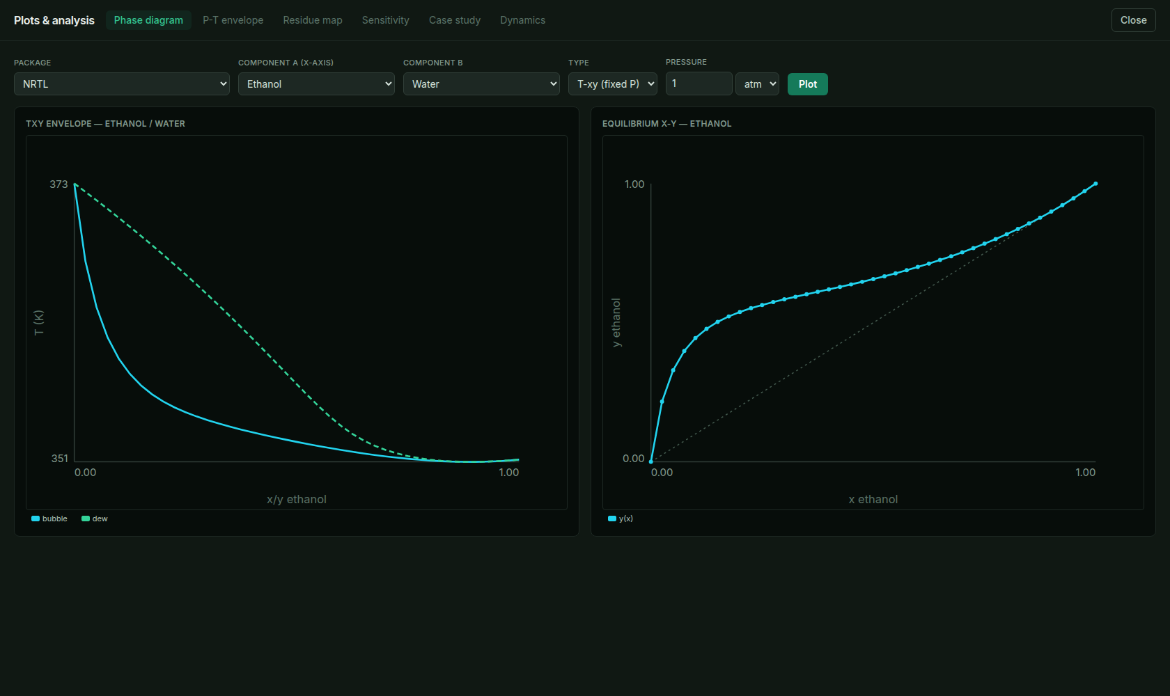
The ethanol-water T-xy phase diagram under NRTL. The bubble/dew curves meet the diagonal at the azeotrope — the ceiling ordinary distillation can't cross. MaximaLabs validates this system against published experimental VLE data.
This is also where trust comes from: MaximaLabs pins the ethanol-water NRTL prediction against published data on its validation dashboard (bubble-point AAD < 0.2 K, azeotrope at x ≈ 0.894 / 351.3 K).
2.7 When a component isn't in the databank
Real work runs into molecules the databank has never heard of. Rather than stop, you estimate the missing pure-component properties from structure — group contribution (Joback) for critical constants and normal boiling point, Ambrose-Walton for vapor pressure. MaximaLabs does this in the Thermo tools panel — Analysis & reports ▸ Thermo tools ▸ Property estimator. Enter the molecular groups (or look the component up by CAS number) and it returns the critical constants, normal boiling point, and acentric factor; the estimated component then drops straight into the same flowsheet:
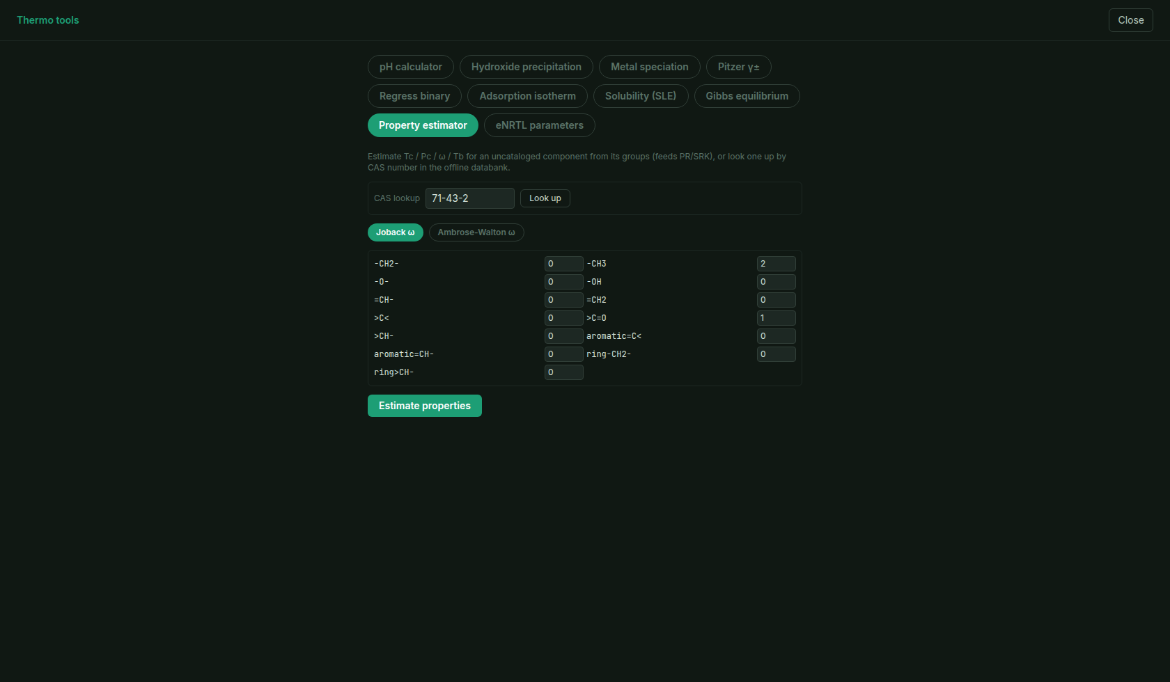
Thermo tools ▸ Property estimator: Joback / Ambrose-Walton group-contribution estimates (or a CAS lookup) for an uncataloged component — critical constants, boiling point, acentric factor — usable in the very next solve.
2.8 Try it: watch the thermodynamics change the answer
- 1Open the ethanol-water distillation example and Run it (it defaults to NRTL). Note the distillate ethanol purity in the stream table.
- 2Click the NRTL pill in the status bar and switch the property method to Peng-Robinson. Watch the recommender flag the mismatch and offer NRTL back.
- 3Run again under Peng-Robinson and compare the distillate purity — the cubic misjudges the azeotrope, so the separation looks different from the NRTL answer.
- 4Open Plots (right rail ▸ Analysis & reports) and generate the Phase diagram for ethanol/water under each package — the azeotrope is there under NRTL and distorted under the cubic.
- 5Switch back to NRTL and re-run to restore the physically correct result.
The lesson of the chapter: the solver from Chapter 1 will faithfully converge whatever thermodynamics you give it — so the property method is yours to get right. Next up, the calculation every one of these models feeds: the flash.
2.9 Exercises
Work each problem yourself first, then reveal the solution to check it. Where a problem says so, reproduce it live in MaximaLabs — the solver is the answer key.
- 1warm-upPick the property method for each and justify in one line: (a) a high-pressure natural-gas mixture of methane, ethane, and propane; (b) an ethanol-water separation at atmospheric pressure.
- 2coreAt an azeotrope, the vapor and liquid compositions are equal (). What does the relative volatilityequal there, and what does that imply for a simple column trying to push ethanol past its ~89 mol% azeotrope?
- 3challengeSuppose you select Peng-Robinson for the ethanol-water column instead of NRTL. Predict what goes wrong, then check it: open ethanol-water distillation and switch the thermo package under the Thermodynamics menu.